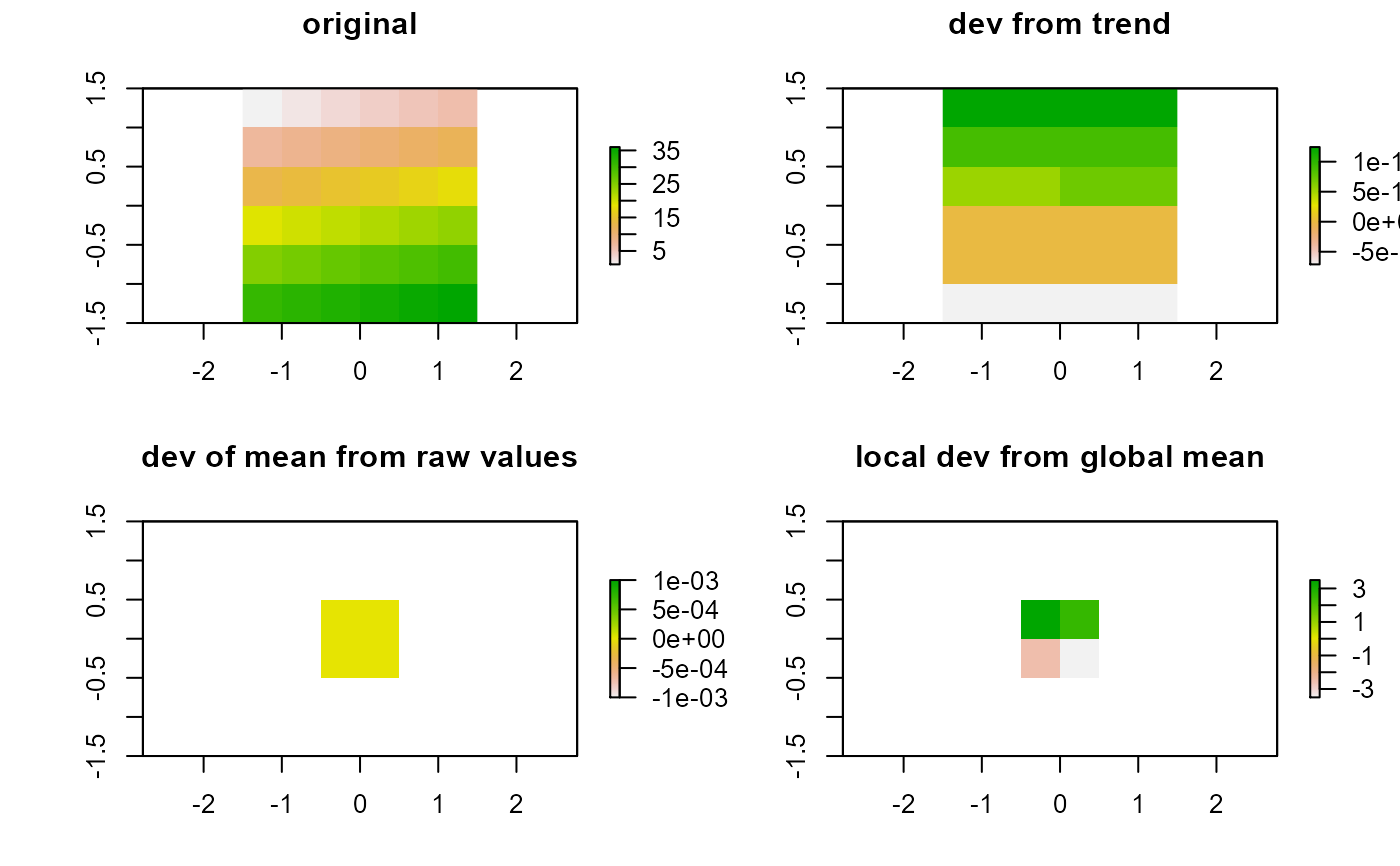
Calculates the local deviation from the raster, a specified global statistic or a polynomial trend of the raster.
The deviation from the trend is derived as [y-hat - y] where; y-hat is the Nth-order polynomial. Whereas the deviation from a global statistic is [y - y-hat] where; y-hat is the local (focal) statistic. The global = TRUE argument allows one to evaluate the local deviation from the global statistic [stat(x) - y-hat] where; stat(x) is the global value of the specified statistic and y-hat is the specified focal statistic.
raster.deviation(x, type = "trend", s = 3, degree = 1, global = FALSE)
Arguments
| x | raster object |
|---|---|
| type | The global statistic to represent the local deviation options are: "trend", "min", "max", "mean", "median" |
| s | Size of matrix (focal window), not used with type="trend" |
| degree | The polynomial degree if type is trend, options are 1 and 2. |
| global | Use single global value for deviation or cell-level values (FALSE/TRUE). Argument is ignored for type="trend" |
Value
raster class object of the local deviation from the raster or specified global statistic
References
Magee, Lonnie (1998). Nonlocal Behavior in Polynomial Regressions. The American Statistician. American Statistical Association. 52(1):20-22
Fan, J. (1996). Local Polynomial Modelling and Its Applications: From linear regression to nonlinear regression. Monographs on Statistics and Applied Probability. Chapman and Hall/CRC. ISBN 0-412-98321-4
Author
Jeffrey S. Evans <jeffrey_evans@tnc.org>
Examples
library(raster) data(elev) # local deviation from first-order trend, global mean and raw value r.dev.trend <- raster.deviation(elev, type="trend", degree=1) r.dev.mean <- raster.deviation(elev, type="mean", s=5) r.gdev.mean <- raster.deviation(elev, type="mean", s=5, global=TRUE) opar <- par(no.readonly=TRUE) par(mfrow=c(2,2)) plot(elev, main="original") plot(r.dev.trend, main="dev from trend") plot(r.dev.mean, main="dev of mean from raw values") plot(r.gdev.mean, main="local dev from global mean")
